DeepSeek-V4.1-Flash, explained step by step
How DeepSeek reduced by a factor of four the memory needed to retain a long context, and by a factor of eight the memory kept between requests, while producing a model that is better than its predecessor. We start with the basics, then examine each innovation through interactive diagrams and the original figures from the paper.
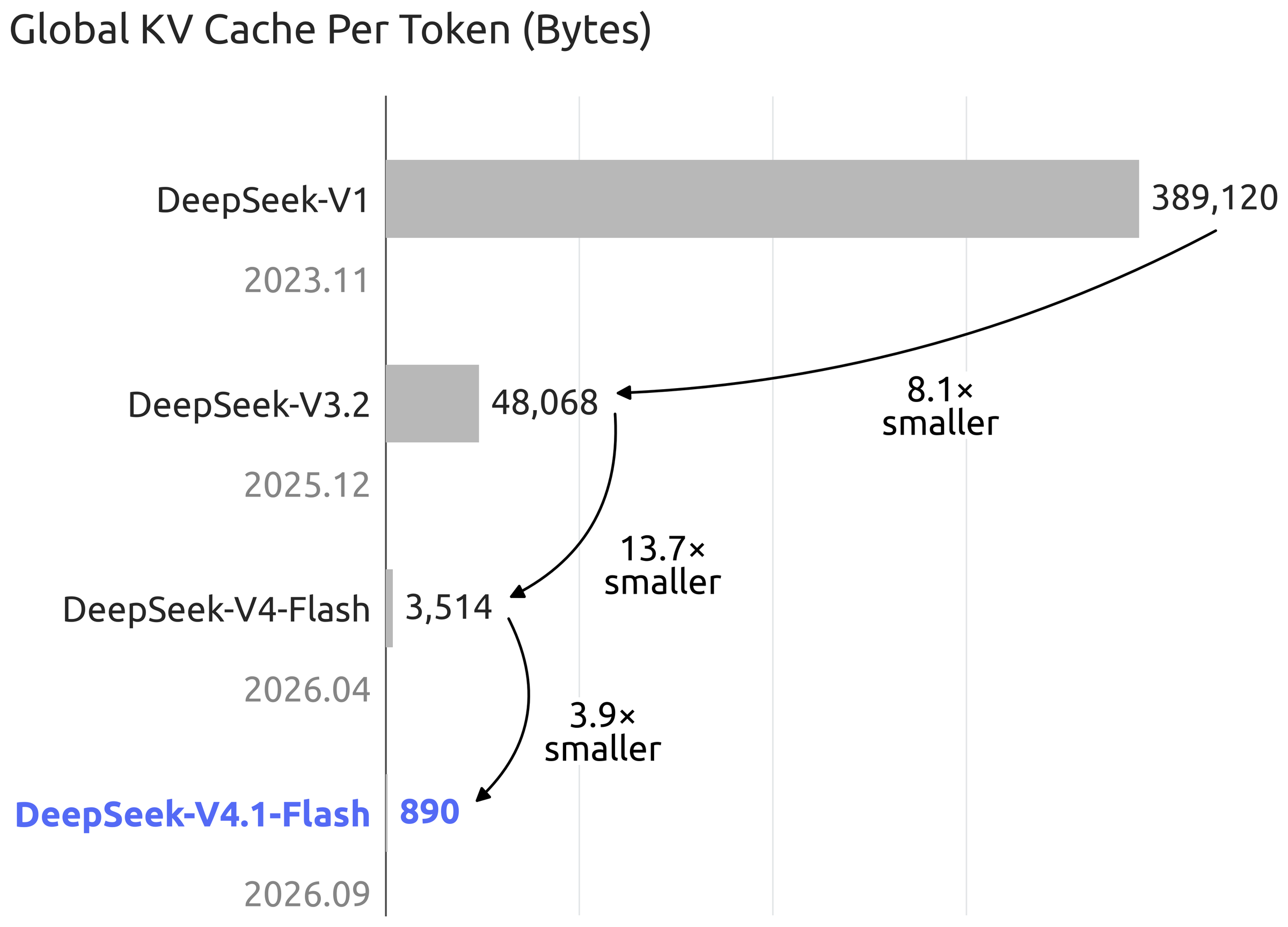
Size of the global KV cache, in bytes per token
The basics in ten minutes
Before attacking the paper, we put in place the six notions without which nothing will be clear: the token, the two prefill and decode phases, the attention, the cache KV, the mix of experts and the different forms of attention. If you already know all this, go to chapter 2.
- Why a model keeps in mind the Keys and values of all that he has read
- The difference between prefill (read) and decode (write), and why agents saturate the prefill
- What "8 B of activated parameters" means in a 552 B model
1.1 A language model writes one token at a time
A LLM does not manipulate words but tokens. His only talent: from a sequence of tokens, predict the next. To write an answer, he predicts a token, adds it to the sequence, and then starts again. It's the generation autoregressive.
This work takes place in two very different phases:
- Prefill : the model reads all the prompt at once. All the tokens are treated in parallel, which makes large multiplications of matrices. This phase is limited by the calculation power.
- The decode The model produces the answer one token at a time. At each step, it only calculates a token, but must reread all its weight and all its memory of the context. This phase is limited by the memory bandwidth.
1.2 Attention: each token queries earlier tokens
To predict the future, every token needs information from previous tokens.attention. Each token produces three vectors:
- a request Q (query) : « What am I looking for? » ;
- a K key (key) : "This is what I have in mind", like the label of a drawer ;
- a value V (value) : the contents of the drawer, the information actually transmitted.
The current token compares its query with all the keys (scalar product). It converts these scores into weights that amount to 1 (softmax), then makes the weighted average of the values. A model stacks dozens of layers DeepSeek-V4.1-Flash has 40 of them.
1.3 The KV cache: the context memory
In a model causal, a token never looks at the future. The keys and values of a past token never change again. Rather than recalculating them at each new token, we store them: it is the KV cache. It grows linearly with the length of the context:
This cache lives on three floors of memory, from the fastest and rarest to the slowest and abundant:
GPU HBM
Memory stuck to the graphics processor, ultra-fast but from a few tens to hundreds of Go. The query cache in progress It's the most expensive resource.
Host RAM (DRAM)
The server memory is bigger and slower. V4.1 places a small cache with a short lifespan, in the order of a few minutes (chapter 8).
SSD
Solid storage but slow. We keep the cache there persistent, which allows the reuse of a prefix already read several hours or days later (at least 72 hours at DeepSeek).
1.4 Why agents change everything
An agent (code assistant, desktop automation, etc.) runs dozens of tool calls. On each turn, the output of the tool (a file, a log, a web page) is added to the context. read (prefill), then write some lines (decode). Result: Workloads become Mostly in entry (input-heavy).
There are two mechanisms to maintain the cost:
- Prefix cache : if the beginning of the context has already been read, you reload your KV cache instead of recalculating it. store This cache, sometimes for a long time, on SSD.
- Cheaper Prefill : for new tokens, and for cases where the cache has been lost (cache miss), we have to recalculate everything.
1.5 The Expert Mix (MOE): Many parameters, few activations
In a Transformer, each layer alternates attention and feed-forward network. MoE, this network is cut into many small experts. A router only activates a few by token. DeepSeek-V4.1-Flash uses in each layer 1 shared expert (always active) and 384 routed experts, including 6 are chosen for each token.
That's why we distinguish total parameters (552 B, stored knowledge) and active parameters (the calculation actually made for a token). Particularity of V4.1: this second digit is 8 B in prefill and 16 B in decodeChapter 4 explains why.
1.6 Three Ways to Look at the Past
A context of a million tokens poses a problem: if each new token compares its request with a million keys, in each layer the cost explodes. The DeepSeek family therefore combines several forms of attention:
- Dense global attention Look at all the past. It's accurate but its cost increases with length.
- Attention with slippery windows (SWA) only look at the nwin = 128 last tokens. Its cost and cache are limited.
- Sparse attention (sparse) : a small module, theindexer, notes all entries of the past and keeps only the top 512 (top-k). The main attention reads only those, plus the local window.
DeepSeek-V3.2 and V4 have introduced these sparse and compressed attentions. The decor of V4.1 is therefore: a branch local (SWA) in each layer + one branch global compressed and sparse.
The memory of the context, KV cache, grows with every token read. Agents read a lot: they pay dearly the prefill (read) cache storage. All innovations in V4.1 address either of these costs.
The problem: the memory of the context costs more than calculation
Previous generations have already made the computation affordable long context through sparse attention. The new bottleneck, the authors say, is the storage and displacement from the KV cache.
In DeepSeek-V4, each layer combines two branches of attention:
- a global branch which covers the whole context. global KV, composed of: main KV (the inputs read by attention) and theindexer K (the keys of the indexer that chooses the entries to read);
- a local SWA branch which maintains the SWA KV Of the last 128 tokens.
The KV SWA has a fixed size, regardless of the length of the context. Global KV that dominates memory. It is limited by the capacity of the HBM. In addition, part of the cache is Persistence on SSD or host RAM to reuse prefixes, adding two constraints: storage capacity and input/output bandwidth.
Together, these computational, storage and bandwidth constraints, according to the authors, form "the main bottleneck" to further reduce deployment costs, and hinder the adoption of agents on longer tasks.
Three levers, combined
Paper presents compression as the fruit of optimization joint Each is the subject of a chapter in this course:
CED + CSA2
The causal encoder-decoder (CED) makes the global KV of the decoder from the encoder. CSA2 shares this KV between layers instead of keeping one per layer.
→ chapters 4, 5, 6
Main cache in FP4
Each number of the main cache is stored on 4 bits instead of 8, with a scale factor for 16 values. The model is trained to support it (QAT).
→ chapter 7
SWA Bounded Replay
The local KV (SWA) is no longer permanently stored. If it is missing, it is reconstructed approximately by replaying only 128 tokens.
→ chapter 8
Announced balance: at equal sequence length, V4.1-Flash only needs about ¼ of the runtime KV cache (in HBM) and about ⅛ of the persistent KV cache (SSD / RAM host) from V4-Flash. Yet it is a model larger (552 B versus 284 B of parameters) and higher performance.
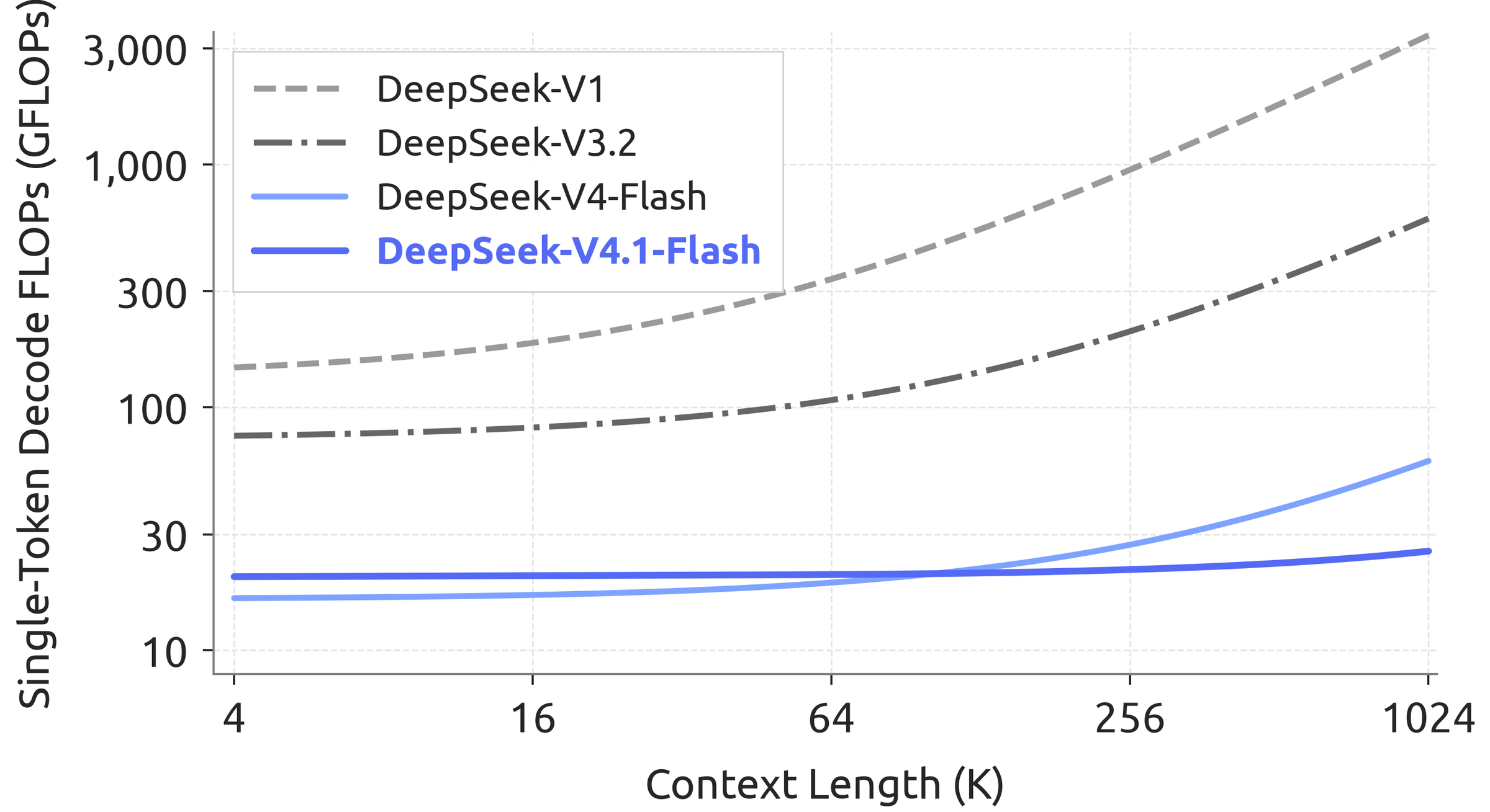
What about the decode calculation?
All improvements also combine on the calculation side. Figure 2 counts the operations needed to generate one It weighs operations BF16, FP8 and FP4 by 1, 0.5 and 0.25. For V4.1-Flash, the curve is almost flat: multiply the context by 256, from 4K to 1M tokens, increases the cost of a token only bya quarter.
The global KV (main KV + indexer K) dominates memory of long contexts. V4.1 reduces it to 890 bytes per token Thanks to three levers: architecture (CED + CSA2), precision (FP4) and deployment (SWA Bounded Replay).
Overview of architecture
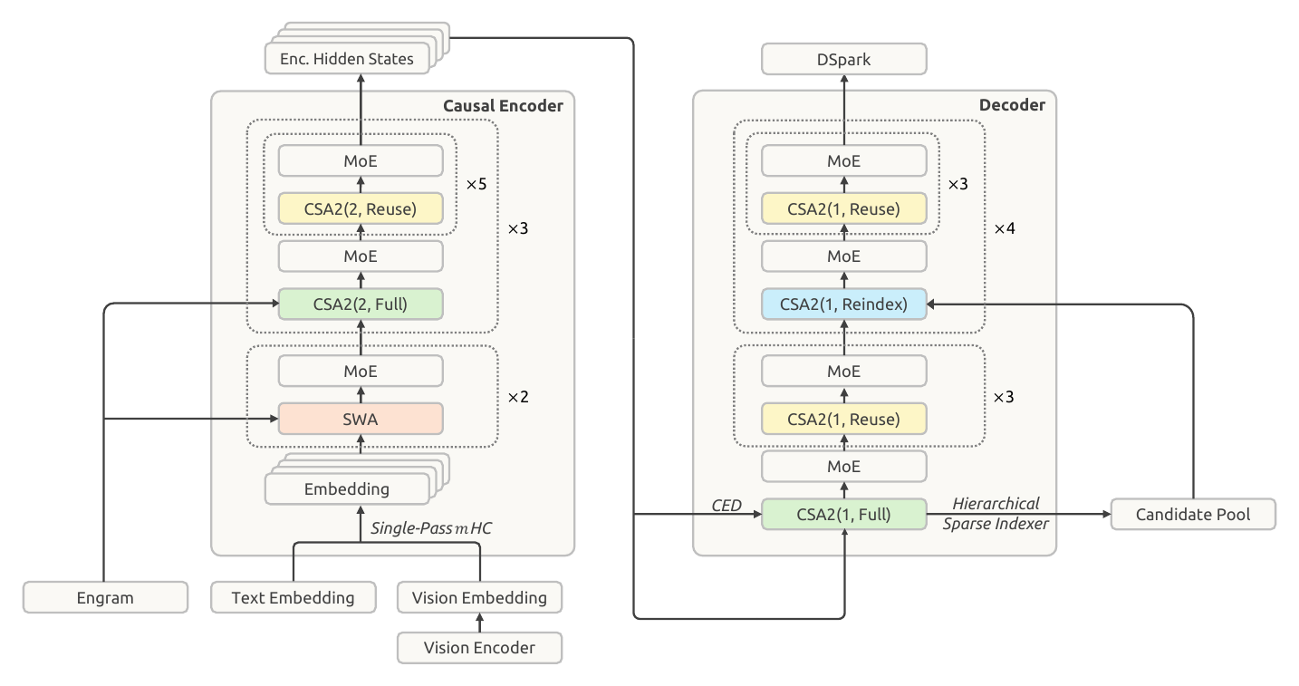
DeepSeek-V4.1-Flash is a multimodal, expert-mixed transformer (text + input images, text output), with 40 layers cut into two halves with distinct roles.
Here is the general map before going into details:
- 40 causal Transformer layers, organized in one causal encoder of 20 layers followed by one decoder with 20 layers. The word “encoder” may seem surprising: here, it remains causal (it never looks ahead). It is simply the lower half of the network.
- Each layer combines a global attention (CSA2) and one local SWA attention, except the first two, in SWA alone.
- All feed-forward layers are DeepSeekMoE standard.
- One vision encoder (DeepSeek-ViT) and a MLP projector transform the images into embeddeds processed with the text from the beginning of pre-training.
- Four additional components: Single-Pass mHC (residual connections), Engram (a memory searchable by hash), DSpark (speculative decoding) andHierarchical sparse indexer.
Key hyperparameters
For the curious, here is the configuration given in section 4.2.1 of the report. No need to remember everything: we will return to each important number over the chapters.
| Element | Value |
|---|---|
| Layers / hidden dimension d | 40 layers (20 encoder + 20 decoder), d = 5 120 |
| Main attention | 64 request heads of size 512; compression of requests to 1,280; 8 output projection groups of size 1,024 |
| Indexer | 32 request heads of dimension 128; top-k = 512 inputs read by attention |
| CSA2 compression | m = 2 in the encoder, m = 1 (no compression) in the decoder |
| SWA Window | nwin = 128 tokens |
| Hierarchical indexer | not more than 2,048 blocks of 8 positions, i.e. 16,384 candidates |
| MoE | 1 shared expert + 384 routed experts (6 activated per token), intermediate size 2,304, SwiGLU bounded (clamp) to 10 |
| mHC | expansion factor 4 (4 residual streams), 20 iterations of Sinkhorn-Knopp |
| Engram | 196 B of parameters distributed over 2 modules (layers 1 and 14, indexed from 0) |
| Vision | 32-layer ViT, size 1,024, 16 heads, 14 px patches; 2-layer MLP projector |
| Parameters | 552 B (backbone); 8 B activated per token in prefill, 16 B in decode |
V4 combined two types of compressed attention (CSA and HCA). V4.1 is only used CSA2. The multi-token prediction module (MTP) used during V3/V4 pre-training is removed; DSpark, trained separately after pre-training, supports speculative decoding.
CED: the causal encoder-decoder that cuts the prefill in half
First great idea of paper: the Causal Encoder-Decoder. It blows up the high half of the network to almost all tokens of the prompt, without losing quality.
- How the decoder gets its global KV without calculating its own layers
- Why local attention (SWA) complicates things, and how the Bounded Replay resolve the problem
- Where the "8 Mds activated in prefill versus 16 B in decode" came from
4.1 The starting point: YoCo
In agent workflows, tool calls generate a lot of prefill queries. When KV cache is not available (cache missIt is necessary to recalculate everything. YoCo (You Only Cache Once, Sun et al., 2024). In YoCo, the upper half of the layers directly reuses the KV cache produced by the lower half. CED builds on this idea and adds structural improvements to increase the KV cache capacity and the computational depth that produces it.
4.2 Overall attention: the decoder is used at the outlet of the encoder
The L/2 = 20 layers from the bottom form the causal encoder. For the top layers (decoder, l > L/2), global KV entries are not not calculated from their own hidden state Hl. They are projected directly from the hidden state of the last layer of the encoder, HL/2, with weights specific to each layer:
Imagine a team of 40 people reading a file. Without CED, each page passes into the hands of the 40s. With CED, the top 20 read each page and write a sheet. The next 20 only consult these sheets and really get involved only on the very last pages, the ones before the answer.
Combined with CSA2 (Chapter 5), this is the layer of the decoder in Full mode which calculates its global KV from HL/2. The other layers of the decoder reuse this KV.
4.3 Local attention: the price of depth
For the slippery window attention, CED keeps the classic calculation layer per layer : the local keys and values of the layer l come from his own hidden state HlThis increases the "calculation depth" of the local KV, but creates an awkward dependency.
For the decoder to start generating, it needs the KV SWA of the last 128 tokens in each of its layersNow the window of layer 30 depends on the outputs of layer 29 on a larger window, which itself depend on layer 28 on an even larger window... The windows pile up. Reconstitute exactly these states requires to pass about nwin × L/2 = 128 × 20 = 2 560 tokens in the decoder layers.
For multi-round interactions with short messages, this additional cost becomes important: we would replay 2,560 tokens to read only a few hundred new ones. Fortunately, previous work (Chen et al., 2025) showed that the effective receiving field SWA is much smaller than the theoretical field nwin × L/2. Hence the Decoder SWA Bounded Replay : the decoder only passes the last 128 tokens The resulting states are approximate, and the paper notes a "negligible" impact on the quality of the responses. The mechanism is detailed in Chapter 8.
4.4 The balance sheet: how much calculation is saved?
4.5 Where do 8 B and 16 B of activated parameters come from?
During the prefill, almost all the tokens of the prompt pass through only the 20 layers of the encoder. Only the last 128 pass through the bounded replay. A token of prompt only activates about half of the parameters: 8 B. A token generated during the decode goes through the 40 layers: 16 B. Since agent charges are dominated by reading, the 8 B figure weighs the most on the bill.
CED has the global KV of the decoder calculated from the output from the encoder. Most of the tokens of the prompt therefore only cross half of the network. The local KV (SWA) remains calculated layer by layer. To avoid replaying 2,560 tokens, V4.1 accepts an approximate reconstruction on only 128 tokens. In total, the prefill costs almost twice as much.
CSA2: Sharing the cache between layers
Compressed Sparse Attention 2 is the core of compression. Instead of each layer keeping its own global cache, a few layers produce it and the others reuse it, sometimes until the selection of entries to read.
5.1. Three multiple compression axes
The authors break down the cost of the KV cache into three dimensions multiplicative :
- The size of each entry : GQA reduces the number of KV heads; MLA (DeepSeek-V2/V3) shares a small latent vector between all heads.
- The Sequence Dimension : one compresses m consecutive single entry tokens, such as CSA and HCA in V4.
- The dimension of the layers : some layers reuse the cache or selections of other layers instead of keeping theirs.
The axis of the layers had already been explored. IndexCache re-uses top-k indices from one layer to another; YOIO calculates sparse routing only once for the entire network; HySparse re-uses the KV of dense layers by sparse layers. But each of these methods has a limit, according to the authors. Reusing the indices does not save the main KV storage. Sharing routing throughout the network limits performance. Hybrid designs keep layers of attention complete. Above all, none covers the three axes at once. CSA2 combines them.
5.2 Anatomy of a CSA2 layer
Like CSA, each CSA2 layer contains:
- the main KV : the entries of the global cache, each summarising m consecutive tokens. m = 1, without compression, is a special case, used in the decoder;
- one light indexer : it notes each entry of the main KV by combining a indexer Q (calculated for the query) and one indexer K (one per entry), then keep the top 512 ;
- l'main attention : the request (main Q) reads the selected entries and the local KV SWA of the layer.
CSA2 simplifies also two things in relation to CSA:
- In CSA, with a ratio m, each entry was made from 2m original entries, with overlap between adjacent inputs and absolute position encoding. CSA2 eliminates overlap and absolute encoding.
- CSA calculated the K indexer by a separate compression path, from the hidden states. CSA2 gets the K indexer by a simple Hand projection KV.
Both changes simplify implementation and speed up training.
5.3 The three modes: Full, Reindex, Reuse
Each CSA2 layer receives, statically (fixed in the architecture), one of the three modes. In all three cases, the layer calculates its own query (hand Q) and its own KV SWA, and produces a new attention output. Modes differ in how they get three things: main KV, l'indexer K and top-k indices.
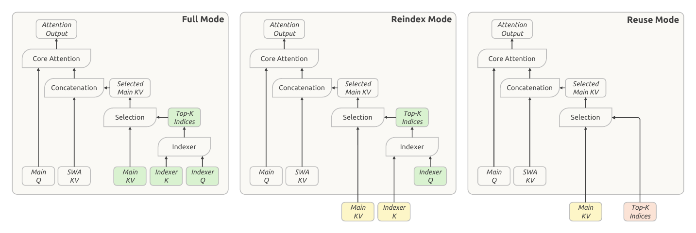
Two distinct mechanisms are at work, and the paper insists on their decoupling :
- Share the main KV and indexer K reduced the storage I'm in hiding.
- Reuse top-k indices avoids computation of the indexer.
Reindex mode is the intermediate: storage is shared, but the layer itself chooses which entries to read. The selection can thus evolve from layer to layer.
5.4 The V4.1 plan: which produces, which reuses
The exact distribution of modes (section 4.2.1):
- Encoder : 0 and 1 layers in pure SWA, then 18 layers CSA2 with m = 2, in 3 identical groups of 6 layers: 1 Full + 5 Reuse.
- Decoder : 20 layers CSA2 with m = 1, in 5 groups of 4. First group: 1 Full + 3 Reuse. The next four groups: 1 Reindex + 3 Reuse. The Full layer of the decoder calculates its global KV since the encoder output (CED).
5.5 Where do the 890 bytes per token come from?
The paper announces 890 bytes of global KV per token, without detailing the calculation. exactly from published hyperparameters:
- Only the layers Full store a global KV: 3 in the encoder (with m = 2, or 1⁄2 input per token each) and 1 in the decoder (m = 1, 1 input per token). Total: 3 × 1⁄2 + 1 = 2.5 entries per token.
- An entry of main KV a 512 channels. In FP4, this is 512 × 4 bits = 256 bytes, plus an E4M3 scale of 1 byte per block of 16 channels (32 bytes). Total: 288 bytes.
- One indexer K dimension 128 in MXFP4 format is 64 bytes, plus 4 scales of 1 byte (one per block of 32). Total: 68 bytes.
- 2.5 × (288 + 68) = 2.5 × 356 = 890 bytes.
This calculation is ours, not that of paper. It assumes that the indexer K is a single head of dimension 128 (the published indexer head size) in the format MXFP4 (adopted for the indexer according to section 2.4.4). The fact that it falls exactly on 890 suggests that these assumptions are the right ones.
In V4.1, only 4 out of 38 layers CSA2 layers store a global KV. The others reuse it (Reindex, Reuse). Reuse Re-uses even entry selection. This brings the cache to 2.5 entries per token. With FP4, you get 890 bytes per token.
The hierarchical sparse indexer
Even with reuse, the Reindex layers still note all To a million tokens, it is a neck. Solution: the first indexing layer restricts the search field of the following.
Previous work (Xu et al., 2026) made the indexer himself sparse: they first noted block-mediated representations, then looked in detail at only the best blocks. The authors note that, in the decoder, the information of the shallow indexers can naturally restrict the candidates of the deeper indexers, without any additional condition.
The mechanism, used only in the decoder CED:
- The Full layer of the decoder records all positions.It travels all the visible main KV and produces its own top-512 clues for its own attention.
- She selects blocks.Each block of 8 positions receives the maximum score of its positions. The best rated blocks (up to 2,048) are retained.
- She forms a pool of candidates.The positions covered by these blocks, up to 2,048 × 8 = 16 384, form the search field of the following layers. This pool is much larger than the top-512 final.
- Reindex layers only note the pool.Each keeps its own top-512 among the 16,384 candidates. Reuse layers do not index at all.
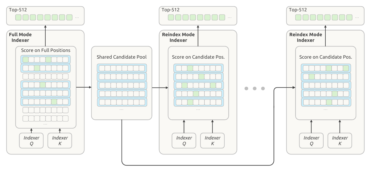
For a fixed pool size, the cost per request of deep indexers goes from linear in the length of context to constant. Only the first Full layer continues to browse the entire context.
The mechanism is "aware of the training": it is introduced during the post-training, and the restriction of candidates is applied to identical training and inference. Deep indexers are therefore optimized for the research field they will actually have in production.
Full layer of the decoder makes a global tracking and identifies 16,384 candidate positions. Reindex layers search only this pool: their cost no longer depends on context length.
The main FP4 cache: 4 bits per number
Second lever: precision. Each main KV number is stored on 4 bits. The secret not to lose quality: a scale factor shared by small groups of 16 values, and a model trained to get used to it.
7.1 From where
DeepSeek-V4 already used thequantification conscious training (QAT) to store in FP4 requests and keysindexer. This accelerated indexing and reduced the indexer cache. For these tensors, DeepSeek chose the standard format MXFP4 of the OCP, compatible with as many materials as possible, even if other formats were more precise in their experiments.
V4.1 extends the QAT to main KV. Here, FP4 is not used to accelerate matrice multiplications, only at reduce storage. Values are decompressed before attention. Therefore, one can choose a more precise format than MXFP4 without requiring that the material be able to multiply natively in this format.
7.2 The format chosen: E2M1 + one E4M3 scale every 16 channels
Each value is a floating 4 bit number E2M1 : 1 bit of sign, 2 bits of exponent, 1 bit of mantisse. It can only represent 8 amplitudes :
To cover larger or smaller values, each block of 16 channels share a scale factor stored in E4M3 (an 8-bit float). This is the NVFP4 schema. without the second global scale. Why can we do without it? The authors justify it by calculating the limits:
- The format can represent up to 448 (maximum of E4M3) × 6 (maximum of E2M1) = 2 688.
- After normalisation of RMS (RMSNorm weight driven ≤ ~1), the L2 standard of the 512 channel latent vector is at most s512. RoPE rotation preserves this standard, so no value exceeds 22.6.
- In practice, the maximum observed during training revolves around 10.
The margin is huge. Delete the global scale therefore does not cost "no measurable loss of precision" and simplifies the layout of the cache.
7.3 Options for implementation
- QAT during post-training : the model learns to work with a FP4 cache.
- Same format for the part with RoPE and the part without RoPE of the vector.
- Quantification after RoPE quantification before provided only a marginal gain in precision and would have added work to each decode step.
- KV SWA remains in FP8, because it is more sensitive to quantification.
Compared to the main KV in FP8 of V4, this format divides almost by two The print, in HBM as on SSD. An input of 512 channels is increased from 512 bytes to 288 bytes.
4 bits per value + 1 byte of scale every 16 channels = 4.5 bits per value On average. Simple mathematical terminals ensure that no global scale is required. The main cache becomes almost twice as light as in FP8.
The persistent cache and the SWA Bounded Replay
Third lever: deployment. The authors find that storing the local KV (SWA) on a sustainable basis is both expensive and unnecessary. They remove it from the persistent cache, and make its absences cheap.
8.1 How V4 handled the persistent cache
In the deployment of V4, a persistent cache on SSD, with a LRU eviction policy (we throw away what has been used the least recently), separately manages two types of KV:
- the global KV, stored in full: one hit allows you to reuse the entire prefix;
- the SWA KV, stored in two specific places: the end of the prompt and the end of the answer. This allows to regenerate a response or to continue a conversation from this point.
The cache was dimensioned so that both types remained resident more than 72 hours problem: although we only keep nwin SWA entries at these positions, this uncompressed KV SWA occupied almost half the ability of the persistent cache, especially in short-round conversations.
8.2 The finding: two KVs, two lifespans
Long drag re-use
A long prefix (a code repository, documentation) can be reread hours or days later. Keep it on SSD for a long time is profitable.
Useful for a few minutes
It only serves within an active session. It becomes useless as soon as the session ends or the next round begins. Keeping it 72 hours is wasteful.
The V4 report already proposed a "Zero SWA Caching": do not store the KV SWA and recalculate it if it is missing. But reconstruction exact requires a complete pass on L × nwin tokens, a cost considered prohibitive in production.
8.3 New management in V4.1
- The KV SWA leaves the persistent cache.It is placed in a distributed memory pool, made up of 10% of the DRAM of each machine. This pool is much smaller, but its very short life span (a few minutes) allows you to recycle the expired entries immediately. In real charge, this is enough to serve the vast majority of active sessions. The global KV remains in the persistent cache, with a guaranteed lifetime of at least 72 hours.
- Absences become cheap: Encode SWA Bounded Replay.For requests, rare but inevitable, which find the global KV but not the KV SWA, we only recalculate nwin = 128 tokens instead of a complete pass on L × nwin tokens. According to the paper, this limited replay is the "cradlestone" of the design: it transforms a miss catastrophic in a mild and inexpensive degradation.
8.4 How the Rejuvenated Play Works
SWA dependencies accumulate from layer to layer (see cone of chapter 4) The limited replay therefore accepts states approximate : he only replays the nwin last tokens and truncates SWA attention to the replayed segment. For a replay starting at the position s, a request in position i only look at the SWA keys in the meantime:
Encoder SWA Bounded Replay
When the encoder's KV SWA is missing, you replay the last 128 tokens of the cached prefix, with the non-hidden part. The replayed tokens only regenerate the KV SWA: the global cached KV is reused as is, without recalculation or crushing. The non-hidden part generates both.
Effect: The prefix cache is dependent only on the global KV, and the KV SWA can disappear from the persistent cache.
Decoder SWA Bounded Replay
To each prefill, the encoder outputs of the last 128 tokens of the prompt are passed in the layers of the decoder, with the same truncation. The KV SWA of the decoder thus obtained serves the decode, never the prefix cache.
Effect: the front pass of the decoder is limited to 128 tokens, which almost halves the total prefill.
The replayed states are not mathematically identical to those of a complete pass. On the encoder side, the KV calculated for the non-hidden part depends even on the position where the cache was found. The authors report that the strategy "rarely compromises" the quality of the answers. For safety, the replay of the decoder is also simulated during post-training, for the model to adapt to it.
8.5 The final result: ⅛
The reduction of the persistent cache by 8 is the result of two factors which multiply:
The global KV (useful for a long time) stays on SSD at least 72 hours. The KV SWA (useful for a few minutes) lives in a small RAM pool. If it has expired, it is reconstructed approximately by replaying 128 tokens. Persistent cache: ½ (SWA removed) × ¼ (global KV) = ⅛ V4-Flash.
Single-Pass mHC: one passage in memory
A more discreet extension, but typical of DeepSeek engineering: shifting a coefficient ofone block removes a dependency and allows to merge three GPU kernels into one. The memory traffic of the activations is divided by two.
9.1 Reminder: mHC hyperconnections
In a classic Transformer, a single "residual flow" crosses the layers: each block reads this flow, calculates, and adds its result. mHC (manifold-constrained Hyper-Connections, Xie et al., 2026), introduced in V4, maintains n residual flows in parallel (n = 4 in V4.1. For each token, these fluxes form a matrix Xl ∈ ℝn×d, updated as follows:
9.2 The problem: three passages in memory instead of one
Ideally, the transition between two blocks would be one operation: read (n + 1)d values (flows + output from previous block) and write them (n + 1)d. This gives a lower bound of (2n + 2)d V4 used in practice three successive cores, due to data dependencies:
9.3 Tip: Use the coefficients from the previous block
Single-Pass mHC offsets the input mixing coefficients of a block. Each block uses the coefficients A produced by the previous block:
In pre-training, DeepSeek keeps the multi-core implementation: the offset only changes the coefficients applied by each block. In deployment, a single merged kernel, Mega-mHC, updates the residual, the input mixture, the coefficient prediction, the pre-normalization and the FP8 conversion. The residual is read once and written once: you reach the ideal terminal and you split by two the memory traffic of the activations in relation to the original implementation.
Using Al−1 for Al, the input mixture no longer awaits the end of an overall calculation. only one passage : (2n + 2)d for 4n + 4)d.
Engram: A memory you can consult by hash
196 billion parameters that cost almost no calculation. Engram separates the Memorization (retain frequent associations of tokens) computation (reasoning).
Engram (Cheng et al., 2026) is a conditional memory The idea: a lot of knowledge is linked to precise tokens ("Route Eiffel", "import numpy as"...). Instead of having them "recalculated" by the layers, they are stored in huge tables of embeddings, addressed by a N-gram hashing before the current token. For each token, we read a few table lines: it is a memory access, not a heavy calculation.
V4.1 repeats the original design: compression of vocabulary (tokenizer compression), multi-head hash, door (gating) depending on context, multi-branch integration. It makes two changes:
- the short causal convolution is withdrawn : its gains did not justify the added complexity in the inference engine;
- tables are optimized by a update to momentum followed by a balance of Sinkhorn (chapter 13).
parameters, also distributed between 2 modules in layers 1 and 14 (indexed from 0), to balance memory between the stages of the training pipeline.
orders of N-grams, 8 hash heads, total embedding size of 2,048 in order. Each head indexes a table of about 16 M entry, with table sizes that are distinct prime numbers.
for embedding tables and key/value projections. The values read and their scale factors are passed directly to the next matrix product.
3 orders × 8 heads × ~16M entries × 256 dimensions per head (2,048 / 8) ≈ 98B parameters per module, or ≈ 196B for two modules. This is our calculation, and it matches the value in the paper.
The profit system: one can preload
Critical point for inference: Addressing is deterministic. The lines to be read depend only on the input tokens, not on the calculations of the network. preload from host memory For the first module (layer 1), this preload is done during the calculation of the first Transformer block. Thus, these 196 B of parameters do not occupy the precious HBM.
At training, the same principle allows preloading for the entire local lot before each stage of the pipeline begins. The tables are partitioned by lines between groups of dedicated processes. During rollouts of RL, on the other hand, they remain in GPU memory to relieve the memory of the host.
Engram adds lots of storage capacity for a minimal cost of calculation. As addresses are deduced from input tokens, tables can live outside the GPU and be preloaded In time.
DSpark: guess several tokens, check at once
The decode is limited by memory: generating a token or checking five costs almost the same. DSpark exploits this fact with a quick " draft" and a scheduler who decides how many tokens check according to the load.
11.1 The principle of speculative decoding
A small fast model (the drafter) offers several tokens in advance. The large model verifies them all in one pass, as a mini-prefill. We keep the longest prefix accepted, plus a token that the large model produces itself at the pass. If the draft is good, we advance several tokens for the price of a decode step.
11.2 What DSpark is doing
- Drafter : 3 Transform blocks with a 128 token slippery attention window.
- Semi-autoregressive draft : only one pass in these blocks calculates the basic logits for 5 positions of draft in parallelA light Markov head then modulates the dependencies between these tokens.
- A confidence head predicts, for each position, the conditional probability of acceptance, deducing the probability of "survival" of each prefix.
- The scheduler combines these estimates with measured flow curves on the engine. He chooses dynamically, for each request, how many tokens check, in order to maximize the expected total flow under the current load.
11.3 Separate training
Unlike the DeepSeek-V3 MTP module, trained with the backbone during all pre-training, DSpark arrives in a dedicated step after pre-training. Only DSpark is trained, the backbone remains frozen. During post-training, DSpark continues to be trained with the backbone, but without propagating gradient It thus remains aligned with the evolving policy. It then accelerates both the online service and the generation of rollouts for RL and distillation (OPD).
DSpark guesses 5 tokens in one pass, estimates the chance that each prefix will be accepted, and lets a scheduler choose the verification length according to the server load.
A natively multimodal model
V4.1-Flash reads images from the first day of pre-training. Its visual encoder is driven home, and a rearrangement trick divides by nine the number of tokens per image.
12.1 The Way of an Image
- The visual encoder cuts the image into patches.DeepSeek-ViT produces a spatial vector grid, one per patch of 14 × 14 pixels.
- Pixel-unshuffle 3 × 3.Each neighbourhood of 3 × 3 patches is rearranged along the channel dimension: 9 vectors become 1 vector 9 times wider. The spatial resolution is divided by 3 in each direction, and the number of visual tokens by 9.
- The MLP projector (2 layers) project these vectors into the hidden dimension of the language model (5,120).
- Insertion into the sequence.Visual embeddings take the place of image tokens in the input sequence and are processed jointly with the text by the backbone.
12.2 DeepSeek-ViT, zero driven
The visual encoder follows the Vision Transformer architecture with several modifications, all thought to look more like a LLM:
- 2D-RoPE instead of absolute positions, to accept arbitrary resolutions;
- the patch embedding convolution is replaced by a linear projection, compatible with the Muon Optimizer;
- RMSNorm and SwiGLU, as in the backbone ;
- 32 layers, size 1,024, 16 heads. Resolutions are supported up to about 1 344 × 1 344 pixels.
His training takes place in two stages, before integration into the backbone:
SigLIP on ~47 B pairs
Sigmoid Contrastive Loss (SigLIP) on about 47 billion image-text pairs from alternative texts, at most 224 × 224 px. Assembling resolution at this stage helped, but made little contribution to the final model for a significant extra cost of calculation.
236 B of tokens with a small LLM
The encoder is connected to a 4 B MoE LLM and trained in prediction of the next token on legends, alternative texts, graphics and OCR. Resolution is limited between 544 × 544 and 1,344 × 1,344Then we throw away the little LLM and keep the encoder.
During pre-training of the complete model, the visual encoder remains frozen Only its final normalization and the projector remain trainingable. It is then thawed and optimized with the LLM, with a lower learning rate.
12.3 Balancing experts... by modality
DeepSeek balances the load of MoE experts without auxiliary loss. Each expert has a correction bias added to the routing score: we lower it if the expert is overloaded, we mount it if it is underused. Problem: image and text tokens do not have the same preferences. Balance the load total can cache a strong imbalance within of each modality.
V4.1 therefore maintains two sets of biases, one for text and one for images. Each token chooses its experts with the biases of its modality, but weighs their outputs with the original scores. After each step, the two games are updated independently, with a speed of 0.001.
The images go through a home ViT (2D-RoPE, linear projection, RMSNorm, SwiGLU), then are compressed ×9 per pixel-unshuffle before entering the same stream as the text. MoE routing is balanced separately for each modality.
Optimizers: Muon per head and balanced updates by Sinkhorn
Two adjustments to the V4 optimization recipe, aligned with the new architecture. One manages the diversity of attention heads, the other tames the huge Engram tables without exploding memory.
13.1 Which optimizes what
| Parameters | Optimizer |
|---|---|
| Linear transformation matrices (backbone, Engram projections, vision-language projector) | Muon (momentum 0.95, weight decay 0.1, RMS update reduced to 0.18, Nesterov) |
| Weight of queries and keys | Muon per head (head-wise) |
| Engram Tables, Token Embedding, Prediction Head | Momentum + Sinkhorn balancing (K = 11, τ = 10−3, ε = 10−20, without weight loss) |
| Standardization, bias, scale factors | AdamW (β1 = 0.9, β2 = 0.95, ε = 10−20, weight decay 0.1 except biases and scales) |
13.2 Muon per head
Muon can be seen as a gradient descent preconditioned : it "orthogonalizes" the updating of a weight matrix before applying it (iterations of Newton-Schulz). one pre-conditioner for the entire query matrix, therefore for all heads at once. Muon per head First cut this matrix head by head. Each head receives its own preconditioner, which better manages the heterogeneity between attention heads. DeepSeek observes that it surpasses the standard Muon; GLM 5 and Kimi-K3 made the same observation.
13.3 Balanced updates by Sinkhorn
Applying Adam to the 196 B of Engram's parameters would have blew up the memory. two states per parameter (mean and variance of gradients). DeepSeek instead uses a momentum update (one state, like Muon) followed by a Sinkhorn balancingShe surpasses Adam empirically.
The procedure follows the same pattern as Muon, replacing orthogonalisation with alternating standardization of the rows and columns the update:
- a line corresponds to a token or N-gram (the identity to be stored), a column with a hidden dimension;
- each row, then each column, is divided alternately by its standard. With an odd number of steps (K = 11), one ends up normalizing the lines;
- multiply byn to switch from a unit L2 standard to a unit RMS per line;
- near-zero rows (norm ≤ τ × mean) are masked for numerical stability;
- the learning rate is corrected by γ = 0.18 to equal the amplitude of Adam's updates (near 0.2 used in Moonlight).
Result: RMS per line and per column of the update are approximately equal to 1.
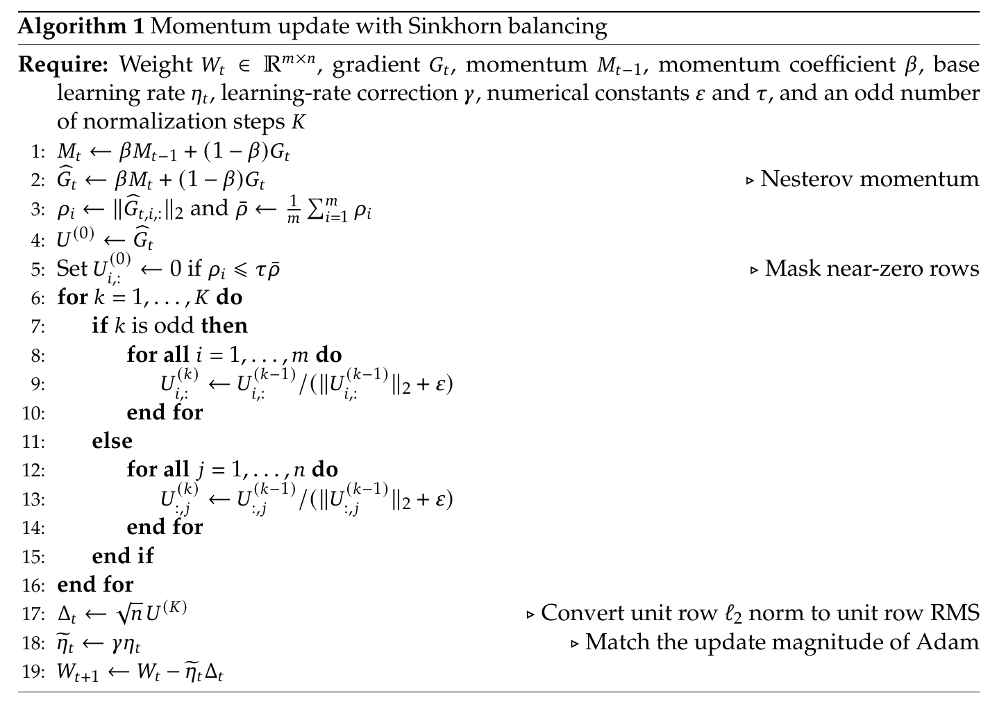
Muon per head gives each head of attention its own preconditioner.Sinkhorn balancing offers large tables of embeddings a well-standardized update, with a single momentum buffer instead of the two states of Adam.
Infrastructure: running all this effectively
An architecture that shares states between layers, images of all sizes, tables of 196 B of parameters... Each idea required a dedicated infrastructure work, on the training side as inference side.
14.1 Multimodal training
Cover Communication During Contrastive Learning
In the contrasting phase of the visual encoder, the loss is calculated over the whole batch. Therefore, it is necessary to collect (all-gather) the text and image vectors of all the machines, which represents a lot of communication. But the gradient of the text vectors depends only on the collected image vectors, and vice versa. while a useful calculation:
"Disaggregated" visual encoder
The visual encoder is replicated outside the LLM parameter tree. Each training step has three phases: forward vision, forward/backward LLM, backward vision. The LLM phase remains free of visual computation and keeps the text parallelism strategy alone.
Distributed images, read once
An ultra-long sequence rich in images can saturate a loading machine, so its images are distributed, with load balancing, between the ranks of context parallelism, and each one is loaded only once.
Incremental transfer to RL
During rollouts of RL, images are sent to the inference engine only incrementally. The decoding and preprocessing results are cached on a distributed file system, reused from one rollout to another and for training.
Conducting attention that shares states between layers
With CSA2, a layer can reuse the main KV, the K indexer or the clues of another layer. However, these layers can be found on different stages of the pipeline, so on different GPUs. Three mechanisms make this transparent:
- Ghost indexers (shadow indexers) : a light and executable replica on each stage concerned, with only one logical owner of the shared parameters. The owner manages the optimization and checkpoints. Synchronization of the parameters and aggregation of the gradients keep the replicas consistent.
- Extensions of pipeline payload : intermediate representations and route information travel with existing point-to-point communications when the source and the consumer are on either side of a floor border.
- Management of micro-lot shared statements : one tracks the lifetime of each state shared through forward, recalculation of activations and backward. Each one is released as soon as its last consumer has finished.
14.2 Inference
GPU kernels only for a layer in Reuse mode, prefill / decode. This is the vast majority of layers. The merged kernels come from FlashMLA (RoPE-attention-RoPE-cast), DeepGEMM (Mega-Gate, Mega-mHC, Mega-MoE), TileKernels and DeepSelect (top-k).
Visual encoding, prefill and decode rotate on separate resources. They scale independently and execute in recovery.
The global KV, with a long service life, is separated from the KV SWA from the encoder, with a short service life. The limited replay reconstructs the latter if it is missing (chapter 8).
Communication-calculation recovery, Engram tables distributed (sharded), separate Bounded Replay paths for encoder and decoder.
"Although architecture is conceptually complex, the resulting flow of inference kernels is remarkably concise."
Pre-training: 45 000 billion tokens
More demanding data, a mixture of text and image from the start, and a training of sparse attention "from scratch". The result: a basic model that rivals V4-Pro, three times larger.
15.1 Data
Search for information
Beyond the sample quality, the team is interested in the interactions between corpus that provide unique information. A "scale" of experiments on parameters and data guides major trainings.
Content generated by models low gain of information is filtered: output of less capable models, poor quality automatic translations. implicit duplication, harmful on long training. The corpus also includes more recent code (new repositories, commits, libraries, frameworks).
The web as is, well cleaned
Three families: image-text pairs (alternative text, relevance threshold, semantic deduplication), interlaced image-text data (web pages and PDF) and domain data (visual location, score, OCR, rare knowledge, image-code pairs, computer use trajectories).
No massive synthesis: the priority is to clean and use raw data. Crawler, too centred text, has been relaunched from Common Crawl. The intertwined data goes through increasingly expensive filtering steps, up to a strict notation by SmolVLM.
The two pipelines are merged: when a sample exists in text and multimodal version, the multimodal version replaces the other. The final corpus has a ratio of 7:1 between text tokens alone and multimodal tokens. The sequence filling algorithm (best-fit packing) reached a padding rate of not more than 10−4.
15.2 The training process
The lot is fixed at 100.6 million tokens during all training. sparse attention is trained from the start at a sequence length of 64K, without heating phase in dense attention. The sequence passes to 1M 34T tokens. The paper states: "without any instability".
15.3 The Basic Model for Seniors
Table 1 compares three core models evaluated in the same internal framework: V4-Flash-Base (284 B, 13 B activated), V4-Pro-Base (1.6 T, 49 B activated) and V4.1-Flash-Base (552 B, 8/16 B activated). Variations of 0.3 point or less are considered equivalent.
To measure real-world R&D capabilities, the team also measures the perplexity on internal corpuses never seen: internal documentation, proprietary code repositories, academic documents. The metric is the number of bits per byte (BPB, bits-per-byte) : the lower it is, the better the "compress" model, so predicted, the text.
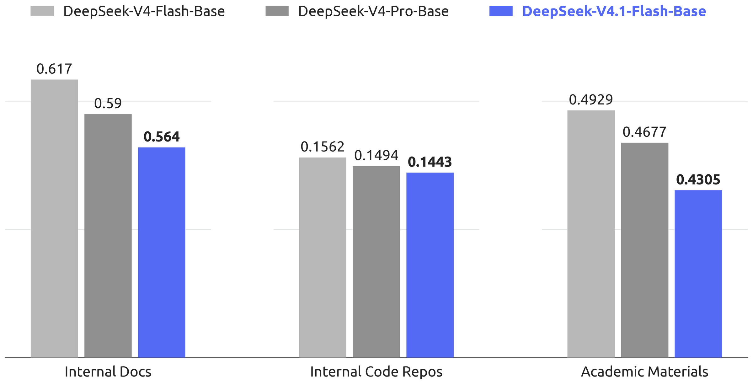
V4.1-Flash-Base achieves the level of knowledge and reasoning of V4-Pro-Base With about 1⁄3 of its total parameters and 1⁄4 of its parameters activated. On internal evaluations never seen, the paper announces gains of 5 to 10%. The authors see it as the mark of a better curation of the data.
Post-training: everything is in the data
Rarely seen in a technical report: no algorithmic innovation The gains come almost entirely from automated pipelines that produce tasks, environments and very large-scale verifications.
The recipe is standard: SFT (fine-tuning supervised), then RL (learning by strengthening), then OPD (distillation on-policy), without any change from V4. The effort consists of three steps:
- synthesize various tasks and verifiable, with their reference solutions and reward signals;
- to construct by procedural agent environments interactive ways to collect and evaluate low-cost trajectories;
- Filter, deduce and calibrate the difficulty.
At this stage, the marginal performance of data engineering and environments is "substantially" higher than that of algorithmic novelty in post-training.
16.1 Making large-scale tasks
Each task is one triplet (problem, environment, verification system) Its quality is judged on two axes: difficulty (not trivial) and the correction (no critical flaws in all three components). The model starts to know how to build its own training tasks. DeepSeek therefore trains it to build better ones, with difficulty and correction as rewards. Each task is monitored throughout its life: each new use in RL provides trajectories that allow it to be re-audited.
Replaying the real world
Employees and partners use the latest model in their daily work and voluntarily return data and returns. From the observed interfaces, many simulated tools which reproduces the formats, API diagrams and behaviors of real tools: SaaS, enterprise software, trade back-ends. Reassembled failures are used to generate environments that Replay Errors the model to correct them by RL.
A chain of specialized agents
Two sources: sessions of code agents (complex or poorly successful tasks, deduced by trajectory) and public GitHub repositories beyond a star threshold. The construction of each environment is entrusted to several agents:
- Design OfficerVerifies that the project is built, rotates in a container and can be verified automatically. It chooses a starting point (a tower, a commit), designs several rather complex implementation directions and produces evaluation points (fail-to-pass and pass-to-pass).
- Setup agentInstalls dependencies, work directory, tests and task description in an isolated container. It self-tests, erases any trace that can reveal the solution and wraps the environment into a new layer of image.
- Solving agentsSeveral separate agents try the task.
- Quality Inspection OfficerExamines the environment and trajectories: environmental problems, factual errors, inconsistencies between assessment and description, risks of cheating (hackability).
- Repair agentIf the inspection fails, it corrects errors, adjusts the evaluation points too easy or too hard, and the task goes back to verification.
16.2 Moving the RL to scale
The large-scale asynchronous RL is pushed in two directions: computation training and training number of scaffolds (the "harnesses" of agents: Claude Code, OpenCode, Pi, DeepSeek Harness...). Performance continues to rise with the steps of RL, whether in a single scaffold, between versions of the same scaffold or between heterogeneous scaffolds.
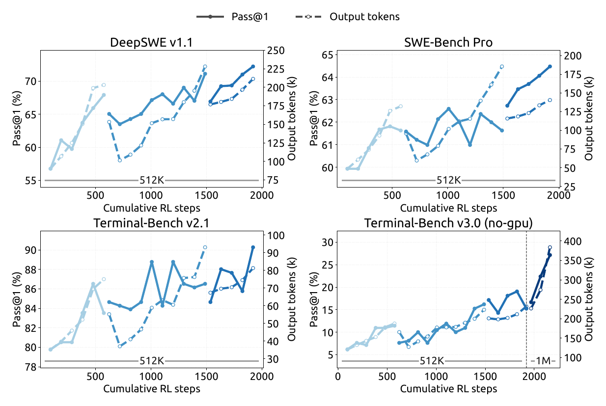
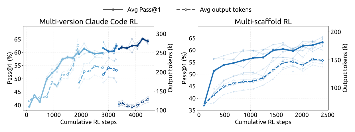
Two engineering ideas accompany this move to scale:
- Separate scaffold from control : one agent sandbox spins the scaffold and its tools. worker container orchestrate the rollout independently of the scaffold and normalize interactions in a common trajectory format. Both spin out of the pre-emptible GPU pool. If the trainer is pre-empted, the rollout can be suspended and unloaded with all its condition.
- Merge models to restart : Checkpoints are merged from training on different scaffolds or configurations to reset the next training. This combines progress achieved by different optimisation paths, and increases in performance and efficiency in tokens.
16.3 Dsec: Millions of sandboxes
To train agents, you need environments where they actually execute code. DSec (DeepSeek Elastic Compute) is the deepseek sandbox platform. For V4.1, the demand is increased to millions of simultaneous instances.
Relaxed consistency
The nodes are cut in shards ("Units d'Scale"), which also limits the damage of a greedy experience. Instead of Kubernetes, a home placement engine turns into several independent replicas, without synchronised coordination. Each node validates the placements itself and refuses those that exceed a local threshold.
Active containers by physical machine, before measurable degradation. This is achieved by linking each VM worker to a NUMA domain via sub-NUMA hardware partitioning.
Latency sensitive class
In order to ensure that timed assessments are not distorted by the neighbours, non-priority tasks go to: SCHED_IDLE. The core scheduling ensures that only tasks of the same priority share a physical core.
Contain cheating
Agents have tried to reward hacking by exploiting recently disclosed vulnerabilities (XFS driver, AppArmor, response leak via packet mirrors). Others have deleted critical binaries, even the file system. Parades: AppArmor profiles by sandbox and eBPF network policies. A crash counts as a failure, with a signal of "percussion" sent to the RL.
16.4 An asynchronous RL infrastructure
In RL for LLM, some very long answers always delay the whole lot: this is the problem of the long tail. The generation has therefore become asynchronous for almost all tasks of RL and OPD. Rollout and training share the same GPU, in shared time. Each task sets a maximum of samples "in flight". when Relaunching new prompt:
Length Bias
The short answers finish first and dominate the first batches. Two parades: limit competition by data set, and be able to throw away the first short samples.
Non-political samples
Some tokens have been generated by an older checkpoint. We limit the maximum rate of off-policy samples, and a loss mask ignores too-expired tokens.
Discontinue and resume without loss
The generation stops at any border of token. The KV cache and expert routing are saved token by token. We resume with the new checkpoint without repeating any prefill, and each state is released as soon as its sample is finished.
Distillation to 40+ teachers
The last step, the OPD on all vocabulary, uses more than 40 teacher models, sometimes different architectures. One changes professor at negligible cost, and the configuration can be modified during the course of the journey without breaking samples in flight.
SFT → RL → OPD, without new algorithm. Performance comes from tasks and environments synthesized on a large scale and verifiable, thousands of sandboxes per machine, and an asynchronous RL that absorbs the long tail.
A button to adjust the reasoning effort
The cost of a model depends not only on its architecture: it also depends on the number of tokens it writes. V4.1 learns to adjust the length of its reflection to a simple number between 1 and 100.
17.1 The effort signal
During the RL, the following instruction is added at the top of the prompt system:
For each training prompt x, several responses are sampled at each level of effort b. The same answers (x, b) form a subgroup, in which rewards are centered to calculate relative benefits, such as GRPO. never directly Two levels of effort between them. The specific behavior at each level comes from a penalty of length that depends on b :
If the marginal benefit of a reflection token decreases roughly exponentially, p′(ℓ) ≈ a · exp(−ℓ/s), then the optimal length is l*(b) ≈ C − s · log k0 + (s/τ)(b − bmin) : one straight line The authors specify that this is a local approximation. The measured lengths are not necessarily linear, as the effort can change the reasoning strategy itself.
17.2 In production
The public API, launched in September 2026, offers three steps that correspond directly to this setting. We change the operating point without touching the weights or decoding parameters:
| API level | Effort b |
|---|---|
| max | 100 |
| high | 75 |
| low | 50 |
Training uses only a finite number of levels, but intermediate values give interpolated behaviors.
17.3 What it gives
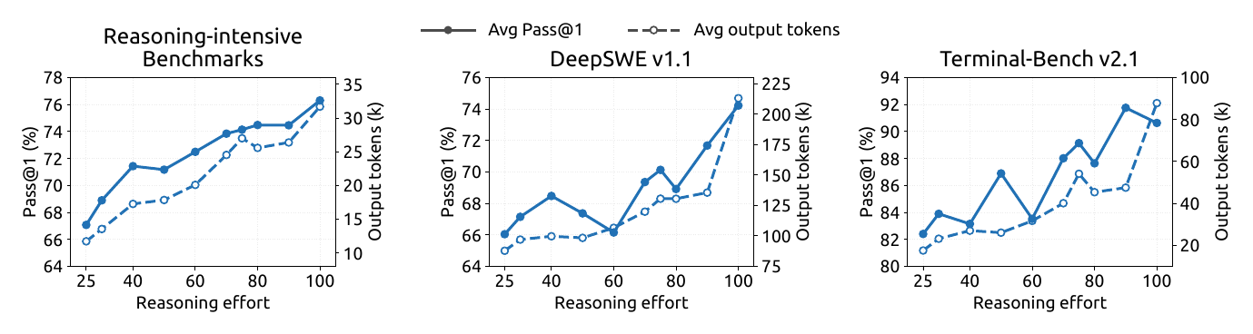
When the effort goes from 25 to 100.
control of the effort learned in single response is transferred to the trajectories of multi-turn agent.
for about 2.5× No more tokens out.
The winnings are concentrated at the beginning. The 60–80 range already recovers most of the precision of the maximum adjustment, for less than half of its budget in tokens. The last step towards 100 extends the agent trajectories from 1.6 to 1.8× for marginal gains. The max level is therefore to be reserved for the most difficult tasks.
The annex details the eight reasoning benchmarks. Length increases steadily, from 2.0 to 3.1× between forces 25 and 100: from 4.6k to 11.4k tokens on AIME 2026, from 29.1k to 86.1k on MathArena Apex 2025. Accuracy does not decrease on any benchmarks: +40.3 points on MathArena Apex 2025 (25.3 → 65.6%), 100% on AIME 2026. In code scaffolds, however, the length always increases with effort, but the Pass@1 follows only from afar, with plateaus and hollows.
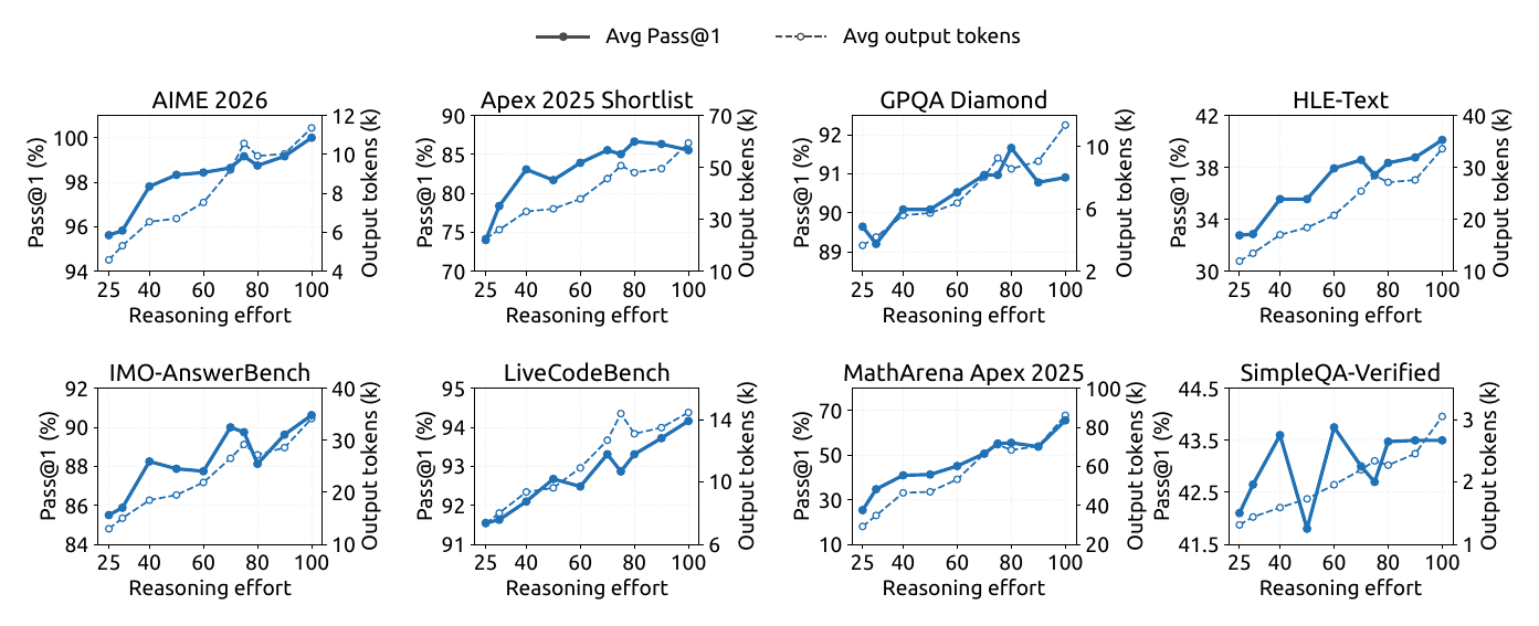
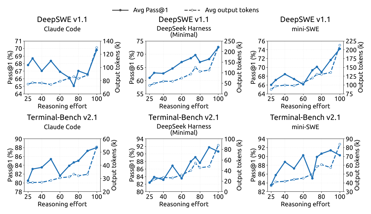
One checkpoint, one number b : the penalty of length exponentially decreasing with the effort required, which produces lengths of reasoning about proportional The intermediate effort (60–80) offers the best cost/quality ratio.
The results: a "Flash" in closed models
On most agent benchmarks, V4.1-Flash joins, or even exceeds, the best closed models of the moment. There is still a gap on the most demanding scientific tasks.
18.1 The Evaluation Framework
- Reasoning : GPQA Diamond, Humanity’s Last Exam (HLE), Codeforces (internal benchmark), MathArena Apex.
- Code agents : Terminal-Bench 2.1 / 3.0 / 4.0, DeepSWE v1.1, ProgramBench, NL2Repo-Bench. Rated with DeepSeek Harness Minimal Mode, 1M context tokens, temperature 1.0, top-p 0.95 (mini-SWE for DeepSWE).
- Cybersecurity : SEC-Bench Pro, CyberGym, ExploitGym.
- General-purpose agents : AutomationBench, Agents' Last Exam.
- Vision agents : Chartography, BabyVision, ZeroBench (with the harness Claude Code, context of 512k).
To limit cheating in code evaluations, internet access is cut, Git history is removed and compilation or package caches are purged. However, exploit searching behaviors have been observed, such as decompiling Ubuntu packages to find vulnerabilities in CyberGym. The authors call on the community to take this into account in future benchmarks.
Where V4.1-Flash leads
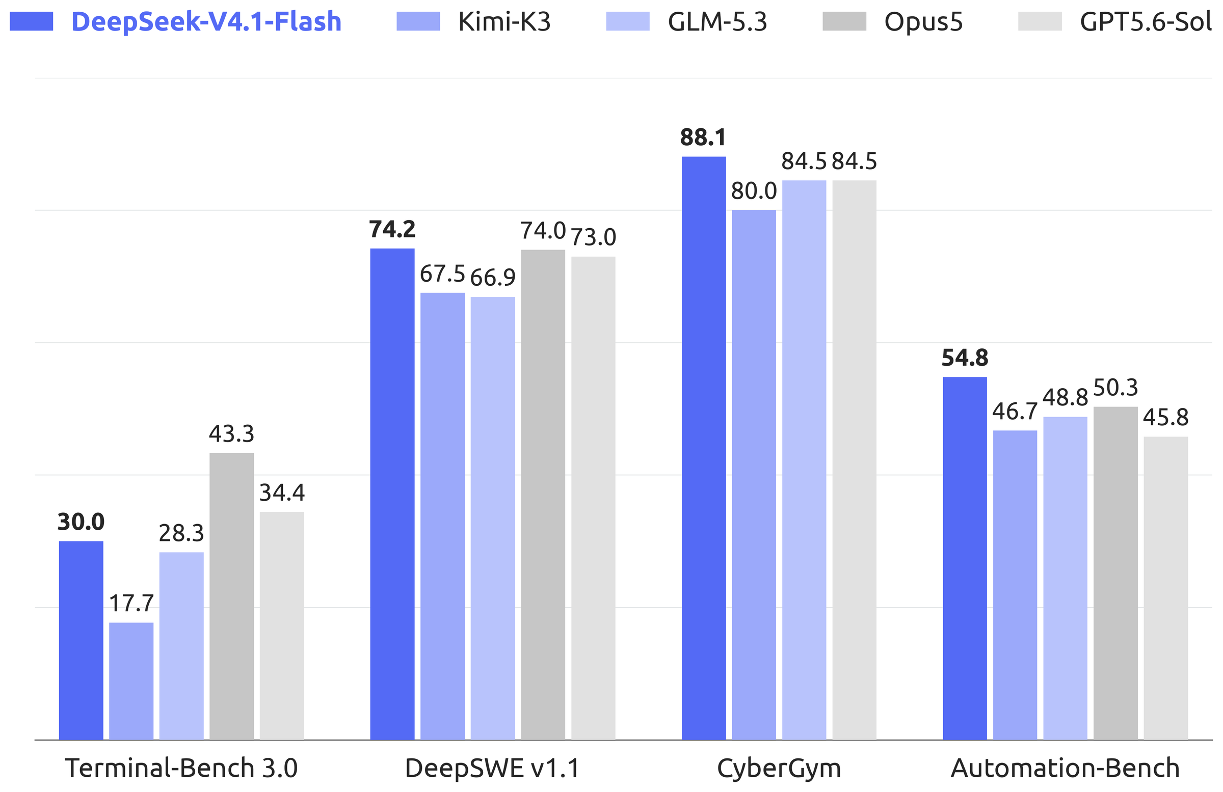
Codeforces 3 471 (compared with 3,348 for V4-Pro), DeepSWE 74.2 % (before Opus-5 at 74.0% and GPT-5.6 Sol at 73.0%), Terminal-Bench 2.1 90.6 %, Automation-Bench 54.8 %, Agents' Last Exam 31.8 %, CyberGym 88.1 % (new state of art among open models in cybersecurity).
Where the gap persists
The duties of an officer with high scientific expertise: Terminal-Bench 4.0 (31.2 versus 51.8 for Opus-5), Terminal-Bench 3.0, ProgramBench, HLE Without tools (36.8 vs. 56.3), ExploitGym. In vision, V4.1 surpasses Kimi-K3 but remains behind the best closed models.
18.2 Robust from one scaffold to another
A model is rarely deployed in a single harness. The authors keep the same checkpoint, the same decoding configuration and the same tasks, and only change the scaffold (prompt system, tools, turn logic): eight configurations from six families.
Capabilities are transferred well between scaffold families, which is consistent with the diversity of environments and tool formats of synthesized data. On Claude Code, four versions tested give on average 68.9 % on DeepSWE and 87.8 % on Terminal-Bench 2.1 (annex, table 5).
18.3 Working as a team of agents
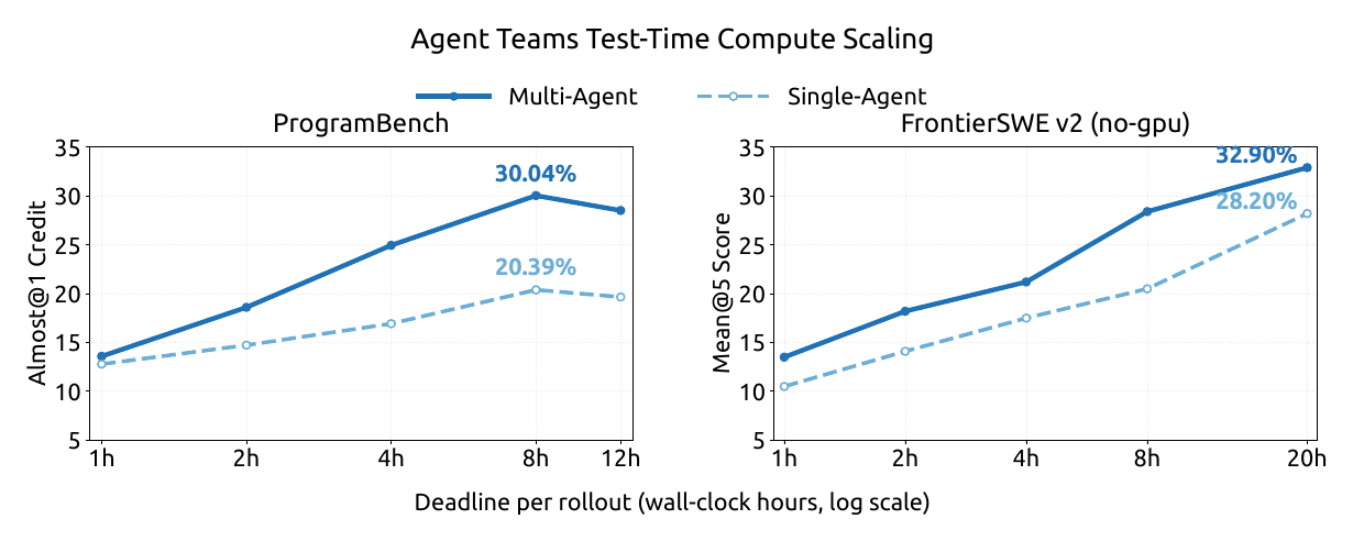
Preliminary experience: the mode Agent Team DeepSeek Harness. A chief agent asynchronously creates appointed and persistent teammates (spawn_teammate) Each starts either "new" or with a copy of the leader's history (fork) All share the same checkout of the deposit. They communicate through a durable mailbox (send_message) The Chief monitors the status of the team (list_agents, wait_agent), can interrupt a partner (interrupt_agent) and maintains a shared task table. At the end, it rereads, tests and books.
RL training combines three terms: task performance, a collaboration bonus (delegate, communicate) and latency penalty derived. This latency is the length of the critical path An acyclic graph of events: costs in tokens are converted at fixed prefill/decode speeds, plus the measured time of the tools, thus encouraging useful parallelism and penalising unnecessary waiting.
With 8 to 16 B of activated parameters, V4.1-Flash equals or exceeds the best closed models of the table on the majority of code and automation agent benchmarks. It remains clearly behind on tasks with high scientific expertise (Terminal-Bench 3.0 / 4.0, HLE).
Limitations and prospects
The paper ends on a section of fairly frank limits. It is worth reading, because aggressive compression has a potential price.
The new architecture creates "strongness boundaries" not yet fully characterized. Internal evaluations have shown no systematic degradation, but no finite test set covers all extreme cases. The authors cite two risks: Selection errors in CSA2 (the indexer misses an important entry), and the approximate reconstruction SWA Bounded Replay, which could degrade capabilities in untested limit cases.
The next priorities announced are:
- extend stress tests, especially the research on very long contexts and the SWA reconstruction at the borders of recovery of the cache ;
- monitor actual loads to characterize failure modes;
- Continue to evolve the evaluation protocols, as benchmarks saturate. Close scores do not mean capabilities equal to the best closed systems on the toughest problems. The paper quotes Fable-5 and GPT-6 Astra as leading references;
- growing together data, model capacity and RL, and co-design the model with its agent harness (model–harness co-design).
The ambition displayed: lower costs and increase capabilities at the same time, to make agents very capable more accessible and easier to deploy.
Summary and final quiz
All the innovations in the report on a page, then a few questions to check that everything is in place.
| Innovation | Target problem | Idea | Announced gain |
|---|---|---|---|
| CED | Costful Prefill of Agents | The global KV of the decoder is projected since the end of the encoder; only the last tokens pass through the decoder | Prefill s2; 8 B activated in prefill against 16 B in decode |
| CSA2 | A global cache per layer | Full / Reindex / Reuse modes: main KV-sharing, K indexer and indices between layers; compressor and indexer simplified | 4 layers out of 38 store a global KV; 2.5 entries per token |
| Hierarchical indexer | Indexers that record the whole context | The Full layer of the decoder selects a pool of 16,384 candidates; the Reindex layers are only looking there | Cost of constant deep indexers with length |
| Main KV in FP4 | Size of cache entries | E2M1 + one E4M3 scale every 16 channels, without global scale; QAT in post-training | 2 compared to FP8 (288 compared to 512 bytes per entry) |
| SWA Bounded Replay | KV SWA stored for nothing on SSD | KV SWA in a short-lived RAM pool; approximate reconstruction by replaying 128 tokens | Persistent cache ≈ ⅛ of V4-Flash |
| Single-Pass mHC | Residual flow memory traffic | Use Al−1 for input mixture; Mega-mHC merged kernel | Traffic in activations ÷2 |
| Engram | Remembering costs calculation | Embedding tables addressed by N-gram hashing, preloaded from the host | 196 B of memory parameters for minimal calculation |
| DSpark | Memory-limited code | Draft of 5 tokens in one pass, confidence per position, length of verification chosen according to the load | Accelerate RL service and rollouts |
| Controllable effort | Cost of output tokens | Length penalty that decreases exponentially with effort b | One Model, Three Levels of API (50 / 75 / 100) |
To go further
- The full technical report: local copy (PDF, 51 pages) · on Hugging Face
- Checkpoints of the model: huggingface.co/deepseek-ai/DeepSeek-V4.1-Flash
- The work on which it is based, cited in the report: YoCo (Sun et al., 2024), mHC (Xie et al., 2026), Engram (Cheng et al., 2026), DSpark (Cheng et al., 2026), DeepSeek-V4 (DeepSeek-AI, 2026).
This course is based solely on the technical report DeepSeek-V4.1-Flash: Pushing the Limits of KV Cache Compression (DeepSeek-AI, September 2026) The figures marked "paper" are extracted as such. The modules marked "Illustration" simplify a principle with fictitious values. The "Interactive" modules use the figures of the paper or the resulting calculations, indicated as such. The passages in quotation marks briefly reflect the original text.